


Stocks in Ounces: Use Python to Calculate Dow/Gold & Nasdaq/Gold Ratios
Over the last ~21 months, the Dow priced in gold (Dow/Gold) slid from roughly 19—20 to about 11, while Nasdaq/Gold fell from ~8—9 to ~5—6. That’s a clear gold-outperformance regime: stocks rose in USD terms, but gold rose faster. In the 200-year context popularized in the “Dow/Gold” lens, today’s ratio near ~11 sits mid-range—far below stock-euphoria peaks (≈19 in 1929, 29 in 1966, 45 in 1999) and far above gold-dominance troughs (≈2 in 1933 and ≈1 in 1980). Translation: the move is meaningful, not extreme; to revisit sub-2 you’d need either a major equity drawdown, a much bigger gold surge, or both.
What pushes the ratio around? Mainly real yields, the U.S. dollar, risk appetite, and policy/geopolitical stress. When real yields fall or policy risk rises, gold tends to lead and the ratio falls. When real yields and the dollar strengthen together, gold cools and the ratio stabilizes or rises. Given the recent gold run, a normal correction or sideways digestion (10—20% type pullback, not a forecast) would be unsurprising unless real yields keep drifting lower and the dollar weakens again.
Rather than guess, treat the ratio like any other time series. In Python, it’s straightforward: use yfinance to fetch DJIA (^DJI), Nasdaq (^IXIC), and gold (COMEX futures GC=F); use pandas to align dates and compute index / gold; and use matplotlib to plot both USD and oz-of-gold views on dual axes. Add 50/200-day moving averages and a rolling z-score to monitor regime changes: below a falling 200-day = gold-favored; a cross back above = equities regaining the upper hand. Correlate the ratio with TIPS real yields and DXY to see which macro lever is in control.
Everything in this article is reproducible (check out the github repo) with three small scripts: one to pull DJIA/Nasdaq (we limit to Mon/Fri closes to keep the dataset tidy), one to pull gold, and one to merge, compute ratios, and render charts. The code is included inline and mirrored in the repo so you can clone, rerun, and extend (e.g., add alerts, alternate symbols, or longer history). This is education, not advice: we’re not predicting gold; we’re showing how to build and interrogate the data so you can see the regime—not just the price.
Disclaimer: This article is for educational and entertainment purposes only. We are not investors, advisors, or offering investment advice. We do not predict where the price of gold will go. We discuss hypotheticals like “if X happens, then Y could follow,” purely to illustrate how to analyze the data.
Why Look at Stocks in Ounces of Gold?
Pricing stock indexes in ounces of gold is a clean way to separate “stocks up because dollars are down” from “stocks up because earnings and multiples improved.” The classic lens here is the Dow/Gold ratio—how many ounces of gold “buy” the Dow Jones Industrial Average.
A helpful long-view reference is David Chapman’s article, “200 Years of the Dow/Gold Ratio” on Mike’s Money Talks: https://mikesmoneytalks.ca/200-years-of-the-dowgold-ratio/
The piece shows:
- Pre-Fed (pre-1913) the ratio mostly ranged ~0.2—5.
- Post-1913 the swings became larger, with peaks favoring stocks (e.g., ~19 in 1929, ~29 in 1966, ~45 in 1999) and troughs favoring gold (~2 in 1933, ~1 in 1980).
- Takeaway: the regime (stocks vs. gold) can flip for years.
We’ll recreate a modern version of that lens using free data and Python, then compare the recent move to that history.
Fetch Historical Gold Price Data
We’ll fetch the gold price for today, and from recent history, using Yahoo Finance (COMEX continuous futures, GC=F) and align it with some DJIA (^DJI) and NASDAQ Composite (^IXIC) data. Then we’ll compute:
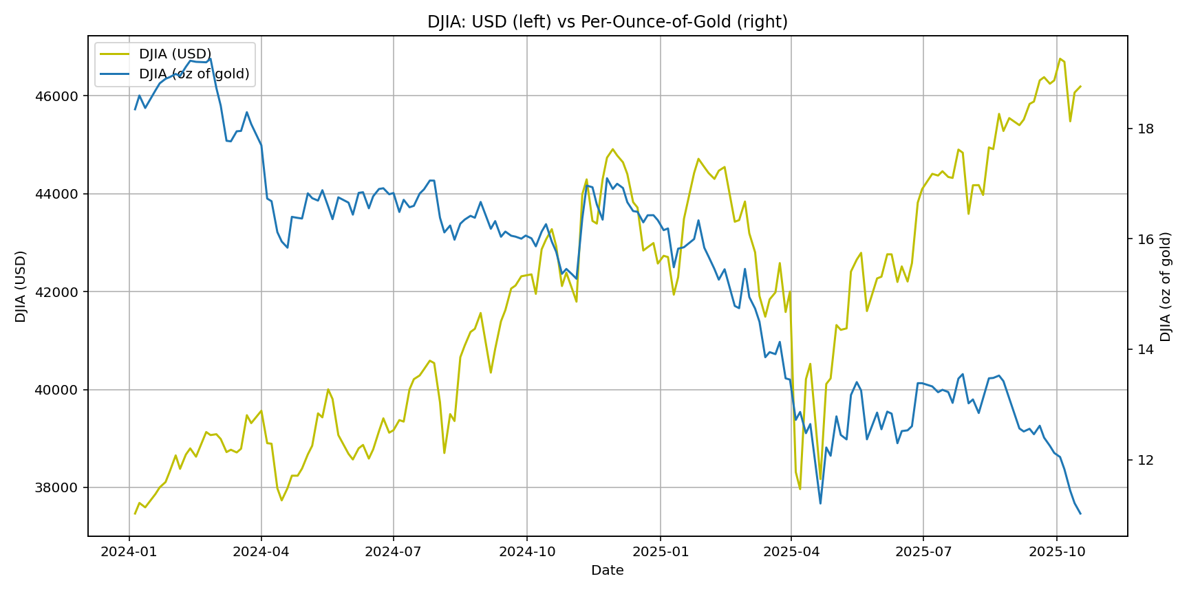
- DJIA (oz of gold) = DJIA(USD) / Gold(USD/oz)
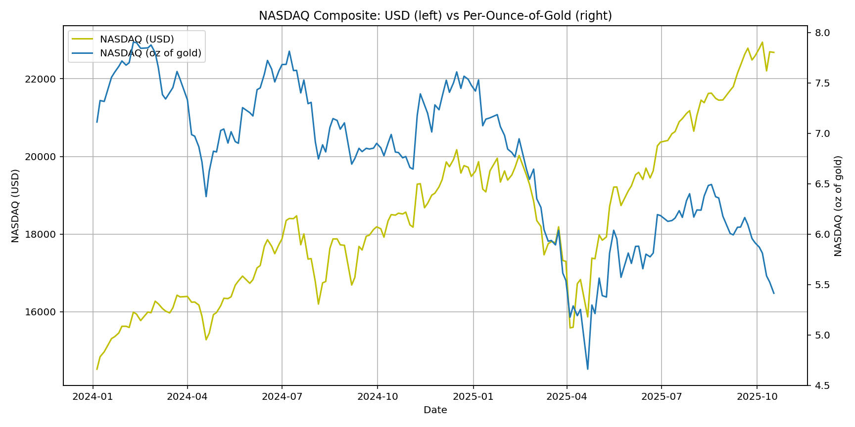
- NASDAQ (oz of gold) = NASDAQ(USD) / Gold(USD/oz)
Finally, we’ll chart USD (left axis) vs oz-of-gold (right axis) for each index so you can see both perspectives at once.
Code, data, and images live here (public repo): https://github.com/basperheim/historic-stock-price-in-gold Feel free to skim the code below, but check the repo for the latest scripts, CSVs, and charts.
Python Data Scripts (free, no paid API)
1) Download DJIA & NASDAQ (Mon/Fri closes only)
historic_stock_data.py
#!/usr/bin/env python3
import time, random
import pandas as pd
import yfinance as yf

START = "2024-01-01"
END   = "2025-10-20"
TICKERS = {"^DJI": "DJI_Close", "^IXIC": "IXIC_Close"}
OUT = f"index_closes_mon_fri_{START}_to_{END}.csv"

def download_range(ticker: str, start: str, end: str, max_retries: int = 4) -> pd.DataFrame:
    delay = 2.0
    last_err = None
    for attempt in range(1, max_retries + 1):
        try:
            df = yf.download(
                ticker,
                start=start,
                end=end,
                interval="1d",
                auto_adjust=False,
                progress=False,
                threads=False  # single-threaded to be gentle
            )
            if df is None or df.empty:
                raise RuntimeError(f"No data returned for {ticker}")
            # Ensure tz-naive index
            if getattr(df.index, "tz", None) is not None:
                df = df.tz_convert(None)
            return df
        except Exception as e:
            last_err = e
            if attempt == max_retries:
                raise
            time.sleep(delay + random.uniform(0, 0.75))
            delay *= 1.6
    raise last_err  # pragma: no cover

def pick_close(df: pd.DataFrame) -> pd.Series:
    s = df["Adj Close"] if "Adj Close" in df.columns else df["Close"]
    # Set the series name explicitly (avoid Series.rename with a string)
    s = s.copy()
    s.name = "Close"
    return s

def filter_mon_fri(s: pd.Series) -> pd.Series:
    s = s.copy()
    s.index = pd.to_datetime(s.index)
    wd = s.index.weekday  # 0=Mon..6=Sun
    return s[(wd == 0) | (wd == 4)]

def main():
    series = []
    for i, (sym, out_col) in enumerate(TICKERS.items()):
        if i > 0:
            time.sleep(2.5)  # small pause between the two requests
        df = download_range(sym, START, END)
        close = filter_mon_fri(pick_close(df))
        close.name = out_col
        series.append(close)

    out = pd.concat(series, axis=1).sort_index()
    out = out.reset_index().rename(columns={"index": "Date"})
    out["Date"] = pd.to_datetime(out["Date"]).dt.strftime("%Y-%m-%d")
    out.to_csv(OUT, index=False)
    print(f"Wrote {len(out):,} rows → {OUT}")

if __name__ == "__main__":
    main()
2) Download Gold (raw daily, tidy to CSV)
historic_gold_price.py
#!/usr/bin/env python3
"""
Fetch raw gold price history and write to CSV (no merging, no transforms).
Primary: 'GC=F' (COMEX Gold continuous futures)
Fallback: 'MGC=F' (Micro Gold futures)

Requires:
  pip install yfinance pandas
"""

import time, random
import pandas as pd
import yfinance as yf

# ---- CONFIG ----
START = "2024-01-01"
END   = "2025-10-20"
SYMBOLS_TRY = ["GC=F", "MGC=F"]  # try in order
OUT_TEMPLATE = "gold_raw_{sym}_{start}_{end}.csv"

def download_yf(ticker: str, start: str, end: str, max_retries: int = 4) -> pd.DataFrame:
    delay = 2.0
    last_err = None
    for attempt in range(1, max_retries + 1):
        try:
            df = yf.download(
                ticker,
                start=start,
                end=end,
                interval="1d",
                auto_adjust=False,   # keep raw OHLC + Adj Close as-is
                progress=False,
                threads=False
            )
            if df is None or df.empty:
                raise RuntimeError(f"No data returned for {ticker}")
            if getattr(df.index, "tz", None) is not None:
                df = df.tz_convert(None)
            return df
        except Exception as e:
            last_err = e
            if attempt == max_retries:
                raise
            time.sleep(delay + random.uniform(0, 0.75))
            delay *= 1.6
    raise last_err

def main():
    used = None
    df = None
    for sym in SYMBOLS_TRY:
        try:
            df = download_yf(sym, START, END)
            used = sym
            break
        except Exception as e:
            print(f"[WARN] Failed for {sym}: {e}")
    if df is None or used is None:
        raise SystemExit("Could not fetch gold data from any symbol in SYMBOLS_TRY.")

    # Tidy index -> Date column
    out = df.copy()
    out.index = pd.to_datetime(out.index).normalize()
    out = out.reset_index().rename(columns={"index": "Date"})
    out["Date"] = out["Date"].dt.strftime("%Y-%m-%d")

    # Ensure standard column order if present
    cols = ["Date", "Open", "High", "Low", "Close", "Adj Close", "Volume"]
    out = out[[c for c in cols if c in out.columns]]

    out_path = OUT_TEMPLATE.format(sym=used.replace("=", ""), start=START, end=END)
    out.to_csv(out_path, index=False)
    print(f"Gold source used: {used}")
    print(f"Wrote {len(out):,} rows -> {out_path}")

if __name__ == "__main__":
    main()
3) Merge + Charts (USD vs ounces of gold)
build_charts.py
#!/usr/bin/env python3
"""
Build DJIA/NASDAQ vs Gold charts:
- Input 1: index CSV with columns: Date,^DJI,^IXIC
- Input 2: gold CSV from yfinance (GC=F or MGC=F), columns: Date,Open,High,Low,Close,Adj Close,Volume
          (It may contain a second header-like row with ',GC=F,...' — this script drops it.)
- Output: merged CSV + two PNG charts (dual y-axes for readability)

Requirements:
  pip install pandas matplotlib
"""

from __future__ import annotations
from pathlib import Path
import sys
import pandas as pd
import matplotlib.pyplot as plt

# ---------- CONFIG ----------
INDEX_CSV = "index_closes_mon_fri_2024-01-01_to_2025-10-20.csv"
GOLD_CSV  = "gold_raw_GCF_2024-01-01_2025-10-20.csv"  # change if your file name differs

OUT_MERGED_CSV = "merged_indices_gold_mon_fri_2024-01-01_to_2025-10-20.csv"
OUT_DJIA_PNG   = "chart_djia_usd_vs_gold.png"
OUT_NASDAQ_PNG = "chart_nasdaq_usd_vs_gold.png"

DJI_COL  = "^DJI"
IXIC_COL = "^IXIC"


# ---------- HELPERS ----------
def require_columns(df: pd.DataFrame, required: list[str], name: str) -> None:
    missing = [c for c in required if c not in df.columns]
    if missing:
        raise SystemExit(f"{name} missing columns: {missing}. Present: {list(df.columns)}")

def load_index_csv(path: str | Path) -> pd.DataFrame:
    df = pd.read_csv(path)
    require_columns(df, ["Date", DJI_COL, IXIC_COL], "Index CSV")
    # Normalize date and enforce numeric
    df["Date"] = pd.to_datetime(df["Date"], errors="coerce").dt.normalize()
    df = df.dropna(subset=["Date"]).sort_values("Date")
    df[DJI_COL]  = pd.to_numeric(df[DJI_COL], errors="coerce")
    df[IXIC_COL] = pd.to_numeric(df[IXIC_COL], errors="coerce")
    return df

def load_gold_csv(path: str | Path) -> pd.DataFrame:
    g = pd.read_csv(path)
    if "Date" not in g.columns:
        raise SystemExit(f"Gold CSV has no 'Date' column. Columns: {list(g.columns)}")
    # Drop the extra symbol row(s) like ",GC=F,GC=F,..."
    g = g[g["Date"].notna() & (g["Date"].astype(str).str.strip() != "")]
    g["Date"] = pd.to_datetime(g["Date"], errors="coerce").dt.normalize()
    g = g.dropna(subset=["Date"]).sort_values("Date")

    price_col = "Adj Close" if "Adj Close" in g.columns else "Close"
    if price_col not in g.columns:
        raise SystemExit(f"Gold CSV missing 'Adj Close'/'Close'. Columns: {list(g.columns)}")

    g["Gold_Close"] = pd.to_numeric(g[price_col], errors="coerce")
    g = g[["Date", "Gold_Close"]]
    return g

def plot_dual_axis(dates, y_left, y_right, title, y_left_label, y_right_label, out_png):
    fig, ax_left = plt.subplots(figsize=(12, 6))
    ax_right = ax_left.twinx()  # secondary y-axis

    ax_left.plot(dates, y_left, label=y_left_label, color='y') # Yellow color for gold
    ax_right.plot(dates, y_right, label=y_right_label)

    ax_left.set_title(title)
    ax_left.set_xlabel("Date")
    ax_left.set_ylabel(y_left_label)
    ax_right.set_ylabel(y_right_label)

    ax_left.grid(True)

    # Single combined legend
    lines_left, labels_left = ax_left.get_legend_handles_labels()
    lines_right, labels_right = ax_right.get_legend_handles_labels()
    ax_left.legend(lines_left + lines_right, labels_left + labels_right, loc="upper left")

    fig.tight_layout()
    fig.savefig(out_png, dpi=144)
    plt.close(fig)


# ---------- MAIN ----------
def main():
    idx = load_index_csv(INDEX_CSV)
    gold = load_gold_csv(GOLD_CSV)

    # Left-join so we keep your Mon/Fri dates from the index file
    merged = idx.merge(gold, on="Date", how="left").sort_values("Date")

    # Fill missing gold prints (e.g., equity holiday / timing mismatch)
    merged["Gold_Close"] = merged["Gold_Close"].ffill()

    # If still missing, abort with a clear message
    if merged["Gold_Close"].isna().any():
        n_missing = int(merged["Gold_Close"].isna().sum())
        raise SystemExit(
            f"Gold_Close still has {n_missing} NaNs after forward-fill. "
            f"Verify GOLD_CSV range and filename."
        )

    # Compute index levels in ounces of gold
    merged["DJI_per_oz_gold"]  = merged[DJI_COL]  / merged["Gold_Close"]
    merged["IXIC_per_oz_gold"] = merged[IXIC_COL] / merged["Gold_Close"]

    # Write merged CSV
    cols = ["Date", DJI_COL, IXIC_COL, "Gold_Close", "DJI_per_oz_gold", "IXIC_per_oz_gold"]
    merged[cols].to_csv(OUT_MERGED_CSV, index=False)

    # Charts (dual y-axes → clearest for different units)
    plot_dual_axis(
        merged["Date"],
        merged[DJI_COL],
        merged["DJI_per_oz_gold"],
        title="DJIA: USD (left) vs Per-Ounce-of-Gold (right)",
        y_left_label="DJIA (USD)",
        y_right_label="DJIA (oz of gold)",
        out_png=OUT_DJIA_PNG
    )

    plot_dual_axis(
        merged["Date"],
        merged[IXIC_COL],
        merged["IXIC_per_oz_gold"],
        title="NASDAQ Composite: USD (left) vs Per-Ounce-of-Gold (right)",
        y_left_label="NASDAQ (USD)",
        y_right_label="NASDAQ (oz of gold)",
        out_png=OUT_NASDAQ_PNG
    )

    print(f"Wrote merged CSV → {OUT_MERGED_CSV}")
    print(f"Wrote chart → {OUT_DJIA_PNG}")
    print(f"Wrote chart → {OUT_NASDAQ_PNG}")


if __name__ == "__main__":
    try:
        main()
    except SystemExit as e:
        print(str(e), file=sys.stderr)
        sys.exit(1)
DJIA & NASDAQ Results
Using Mon/Fri closes from 2024-01-01 → 2025-10-17:
- DJIA rose in USD, but DJIA per oz of gold fell from roughly ~19—20 to ~11.
- NASDAQ USD rose strongly, yet NASDAQ per oz of gold slid from ~8—9 to ~5—6.
In other words, gold outperformed stocks over this window—even while stocks looked fine in USD terms.
Charts (hosted from the repo):
- DJIA (USD vs oz of gold)
- NASDAQ (USD vs oz of gold)
How the Gold Price Today Lines Up Historically
From the historical pattern in the Chapman article:
- Peaks favoring stocks (≈19 in 1929, 29 in 1966, 45 in 1999) often preceded multi-year stretches where the ratio trended lower (gold > stocks).
- Troughs favoring gold (~2 in 1933; ~1 in 1980) were extreme episodes, not everyday events.
Where are we now? With a ratio near ~11, we’re mid-range by post-WWII standards: far below euphoric stock-favoring peaks, still well above deep gold-favoring troughs. The most recent move—your charts show this clearly—has been a meaningful leg toward gold, but not an extreme.
What Could Push the Ratio Next (no predictions)
Again—no forecasts. But the ratio is very sensitive to a few macro levers:
-
Real yields (TIPS)
- If real yields rise and stay high, gold often cools → ratio can rise (stocks > gold).
- If real yields fall, gold tends to strengthen → ratio can fall (gold > stocks).
-
USD (DXY)
- A stronger USD is usually a headwind for gold → ratio support.
- A weaker USD helps gold → ratio pressure.
-
Risk appetite & breadth
- Broad earnings growth and multiple expansion favor stocks → ratio up.
- Geopolitics, liquidity stress, or fiscal concerns often favor gold → ratio down.
Hypotheticals, not advice:
- If real yields drift higher and USD firms, a gold correction or sideways pattern would be normal; the ratio could stabilize or bounce.
- If real yields roll over and USD softens while risks stay elevated, the ratio could grind lower even if indexes hold up in USD terms.
How to Extend this Analysis Yourself
- Add 50/200-day moving averages and a rolling z-score to the Dow/Gold and Nasdaq/Gold series.
- Watch for a cross back above the 200-day in the ratio (often the early tell that stocks are regaining the upper hand).
- Correlate the ratio vs 10y TIPS and DXY to see which lever is really driving your window.
Use something like merged_metrics.py to make this data actionable: compute moving averages and z-scores on the Dow/Gold and Nasdaq/Gold ratios, then render a compact dashboard as a PNG image.
What it does
- Builds 50/200-day MAs; flags gold-favored regimes when the ratio is below a falling 200-day, and equity-favored when it crosses back above.
- Computes a rolling z-score (e.g., 3—5 years) to highlight stretched conditions (|z| ≥ 1, 2).
- Exports a single PNG with two small panels (Dow/Gold, Nasdaq/Gold), each showing the ratio, MAs, and shaded ±1/±2 z-bands.
How to implement (minimal sketch)
# merged_metrics.py
import pandas as pd, matplotlib.pyplot as plt

df = pd.read_csv("merged_indices_gold_mon_fri_2024-01-01_to_2025-10-20.csv", parse_dates=["Date"])
df.set_index("Date", inplace=True)

def with_metrics(s: pd.Series, lookback=750):
    out = pd.DataFrame({"ratio": s})
    out["ma50"]  = out["ratio"].rolling(50).mean()
    out["ma200"] = out["ratio"].rolling(200).mean()
    roll = out["ratio"].rolling(lookback, min_periods=252)
    out["z"] = (out["ratio"] - roll.mean()) / roll.std()
    return out

dj = with_metrics(df["DJI_per_oz_gold"])
ix = with_metrics(df["IXIC_per_oz_gold"])

def panel(ax, m, title):
    ax.plot(m.index, m["ratio"], label="ratio")
    ax.plot(m.index, m["ma50"],  label="MA50")
    ax.plot(m.index, m["ma200"], label="MA200")
    for z in (1,2):
        ax.fill_between(m.index,  z, -z, where=(m["z"].notna()),
                        alpha=0.08, step="pre", label=None)
    ax.set_title(title); ax.grid(True); ax.legend()

fig, axs = plt.subplots(2, 1, figsize=(12,8), sharex=True)
panel(axs[0], dj, "Dow/Gold")
panel(axs[1], ix, "Nasdaq/Gold")
plt.tight_layout(); plt.savefig("metrics_dashboard.png", dpi=144)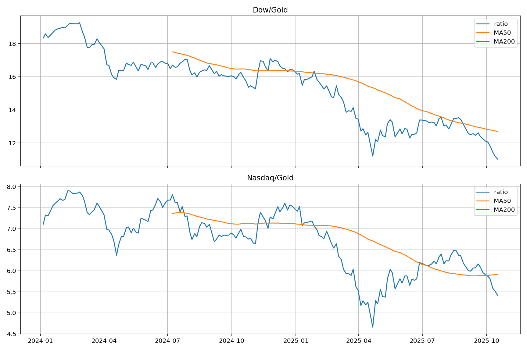
What it looks like
- Two stacked charts with the ratio line, MA50/MA200 overlays, and faint ±1/±2 z-bands.
- Readers immediately see regime shifts (MA crossovers) and extremes (z-score pierces).
Optional upgrades
- Add simple signals (e.g., boolean columns for “ratio < MA200 and MA200 falling”).
- Overlay or annotate DXY and 10y TIPS to show which macro lever aligns with turns.
- Accept CLI args for date range/window sizes so others can reproduce with different horizons.
Conclusion
Pricing indices in ounces of gold turns a noisy “stocks up/down” story into a regime story. This recent dataset shows a clear rotation toward gold—the ratio roughly halved—yet we’re still nowhere near the historical gold-dominance troughs from the 1930s or 1980. The next leg likely depends on real yields (see the 10-year TIPS real yield series at FRED), the USD (DXY) chart (or the trade-weighted USD at FRED), and risk appetite/commodity risk—for background, see Commodity Risk (Investopedia) and the World Gold Council’s research hub—more than on any single headline.
If you find this framework useful, clone the repo, run the scripts, and tweak the dates or symbols: https://github.com/basperheim/historic-stock-price-in-gold
You’ll learn more in a weekend building your own ratios than in a month of scrolling market hot takes.